Method for Reading Thermistors
The thermistor model, jupyter notebook and C++ code I used is available here.
Introduction
So you’re using a thermistor to measure temperature and need to digitize it. Let’s assume you’re trying to get an accurate temperature reading in real units (I’ll use kelvin for that scientific flair). Let’s see how good we can make this measurement.
Thermistors have been around for a long time which usually means we should start by looking in The AoE and browsing EDN’s old issues.
Thermistors aren’t the only temperature sensor by far. Bonnie Baker’s series on EDN is worth a read when choosing a device.
The late, great Jim Williams has an interesting article on some unconventional methods for reading out temperature sensors also on EDN. I particularly like the idea of using an oscillator circuit and getting the resistance from the period.
Modeling Thermistor Data
For this discussion I chose a TDK NTCG103JX103DT1 which with a 0.5% tolerance is one of TDK’s nicer options.
TDK’s product page has measurement data for the min/max/nominal resistance readings over temperature which I’ll use for to following analysis.
P/N,NTCG103JX103DT1,,,,,
R25,10,k +/-,0.5,%,,
B25/85,3435,K  +/- ,0.7,%,,
 ,,,,,,
Temp,Min,Nom,Max,B25/T, -dT,dT
-40,183.7,188.5,193.4,3140,-0.4,0.4
-39,174.1,178.6,183.1,3144,-0.4,0.4
-38,165.1,169.2,173.5,3148,-0.4,0.4
...
From the Min/Max we see that the variability of a single device is low compared to the unit to unit variation. Even a part with 0.5% tolerance like the TDK NTCG103JX103DT1 shown, has significant variation in calculated temperature compared to the nominal value. The temperature difference is calculated by modeling the nominal response using the Steinhart-Hart equation fit discussed below and calculating temperature which would be measured with the min/max tolerance parts.

Tolerance error range in resistance for a TDK NTCG103JX103DT1.

Tolerance error range in temperature for a TDK NTCG103JX103DT1.
Common thermistor models are the Beta model:
\[ T2(R) = \frac{T1}{1 - \frac{T1}{B} \times ln(\frac{R1}{R})} \]and the Steinhart-Hart equation:
\[ T(R) = \frac{1}{A + B \times ln(R) + C \times ln(R)^3}. \]If you don’t care much about precision you can also just use the provided B value but we are using this for a temperature measurement so let’s try and do better than that.
# ------------------------------
# Utility: Steinhart-Hart Model
# ------------------------------

def steinhart_hart_lnR(R: float, A: float, B: float, C: float) -> float:
    lnR = np.log(R)
    return A + B * lnR + C * lnR**3

def fit_steinhart_hart(resistances_ohms, temps_celsius, p0=None):
    """Fit Steinhart-Hart model to resistance and temperature data."""
    temps_kelvin = np.array(temps_celsius) + CELSIUS_TO_KELVIN
    inv_temps = 1.0 / temps_kelvin
    resistances = np.array(resistances_ohms)

    p0 = p0 or [1.0e-3, 2.0e-4, 1.0e-7]  # reasonable guess
    popt, _ = curve_fit(steinhart_hart_lnR, resistances, inv_temps, p0=p0, maxfev=100000, check_finite=False)
    return tuple(popt)  # A, B, C


# ------------------------------
# Utility: Beta Model
# ------------------------------

def beta_model(R, B, T1=25 + CELSIUS_TO_KELVIN, R1=10e3):
    return T1 / (1 - T1 * np.log(R1 / R) / B)

def fit_beta_model(resistances_ohms, temps_celsius, p0=None):
    """Fit beta model to resistance and temperature data."""
    temps_kelvin = np.array(temps_celsius) + CELSIUS_TO_KELVIN
    p0 = p0 or [3500.0]
    popt, _ = curve_fit(beta_model, resistances_ohms, temps_kelvin, p0=p0, maxfev=100000, check_finite=False)
    return popt[0]

# ------------------------------
# Steinhart-Hart Thermistor Class
# ------------------------------

class Thermistor:
    def __init__(self, A: float, B: float, C: float, R0: float = 10_000):
        self.A = A
        self.B = B
        self.C = C
        self.R0 = R0

    def resistance_to_kelvin(self, R: float) -> float:
        inv_T = steinhart_hart_lnR(R, self.A, self.B, self.C)
        return 1.0 / inv_T

    def resistance_to_celsius(self, R: float) -> float:
        return self.resistance_to_kelvin(R) - CELSIUS_TO_KELVIN

    def celsius_to_resistance(self, T_C: float) -> float:
        T_K = T_C + CELSIUS_TO_KELVIN
        return self.kelvin_to_resistance(T_K)

    def kelvin_to_resistance(self, T_K: float) -> float:
        def f(R): return self.resistance_to_kelvin(R) - T_K
        R_guess = np.exp(1/T_K - self.A)/self.B * 0.25
        R_solution, = fsolve(f, R_guess, maxfev=100000)
        return R_solution

# ------------------------------
# Beta Model Thermistor Class
# ------------------------------

class ThermistorBetaModel:
    def __init__(self, B: float, R1: float = 10_000, T1: float = 25 + CELSIUS_TO_KELVIN):
        self.B = B
        self.R1 = R1
        self.T1 = T1

    @staticmethod
    def calc_B(R1, R2, T1, T2):
        return T1 * T2 / (T2 - T1) * np.log(R1 / R2)

    def kelvin_to_resistance(self, T_K: float) -> float:
        exponent = self.B * (T_K - self.T1) / (self.T1 * T_K)
        return self.R1 * np.exp(exponent)

    def resistance_to_kelvin(self, R: float) -> float:
        return self.T1 / (1 - self.T1 * np.log(self.R1 / R) / self.B)

    def resistance_to_celsius(self, R: float) -> float:
        return self.resistance_to_kelvin(R) - CELSIUS_TO_KELVIN


df = pd.read_csv("./ntcg103jx103dt1.csv", skiprows=4)
resistances = df["Nom"] * 1e3  # Nominal resistance in ohms
temps_c = df["Temp"]           # Temperature in Celsius

# Steinhart-Hart Fit
A, B, C = fit_steinhart_hart(resistances, temps_c)
therm_sh = Thermistor(A, B, C)
print(f"Steinhart-Hart coefficients:\nA={A:.6e}, B={B:.6e}, C={C:.6e}")

# Beta Fit
B_val = fit_beta_model(resistances, temps_c)
therm_beta = ThermistorBetaModel(B_val, T1=25+CELSIUS_TO_KELVIN)
print(f"Beta model B value: {B_val:.2f}")

Fit comparison of the Beta model and the Steinhart-Hart equation using a TDK NTCG103JX103DT1.
Steinhart-Hart gives an error significantly lower than the uncertainty of the thermistor. Both models are reasonable within the thermistor variation around the calibration point of the thermistor. To improve absolute accuracy we will need to calibrate our devices.
Calculation
So now we have a way to model the temperature-resistance curve of a given thermistor. Now need a circuit topology to actually measure the resistance and an algorithm to calculate the temperature on actual hardware.
Topology
There are tons of creative ways to approach this including linearizing the thermistor in analog first and skipping the code as well as the afore mentioned oscillator to timer input method.
For this discussion I chose a basic voltage divider (see figure below) with the analysis in software. If we connect the circuit to divide the ADC reference then the conversion is ratiometric, removing error in a voltage transformation from introducing temperature error. We can then skip volts and use the ADC LSB as our unit being divided. More on that in a bit.
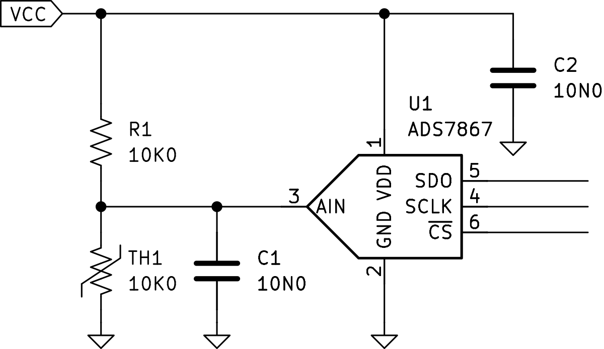
Ratiometric thermistor voltage divider schematic.

ADC Reading of the ratiometric divider topology.
Embedded Calculation
For the embedded calculation we want something that’s got a small code size, is quick to run, and maintains the accuracy we need. We could calculate the logarithm, approximate the logarithm, or use a lookup table (LUT).
Examples of how to use a thermistor often just use the standard library’s floating point natural logarithm but this can take hundreds of clock cycles. Although this may be fine we can do better.
Here’s what I’m looking for:
- constexpr lookup table generated at compile time
- Lookup table error under 0.1% so it doesn’t dominate even with calibration
- Fixed-point values to avoid floating point
If we need to calibrate the table for each board then we can store the LUT in flash or an EEPROM.
Since we have a ratiometric circuit we’ll use ADC values as the index and temperature as the values. The table will be sorted which lets us use a binary search and interpolate between neighboring points.
I’ll first model this in python and then move to C++.
Python Model
def bisect_left(a, x):
    """
    Locate the insertion point for `x` in `a` to maintain sorted order.
    """
    lo = 0
    hi = len(a)
    while lo < hi:
        mid = (lo + hi) // 2
        if a[mid] < x:
            lo = mid + 1
        else:
            hi = mid
    return lo


def interpolate(x_vals, y_vals, x):
    """
    Linearly interpolate to find y for a given x, using x_vals and y_vals.
    """
    if not (len(x_vals) == len(y_vals) and len(x_vals) >= 2):
        raise ValueError("x_vals and y_vals must be the same length and contain at least 2 points")

    i = bisect_left(x_vals, x)

    # Clamp to edges
    if i == 0:
        return y_vals[0]
    if i == len(x_vals):
        return y_vals[-1]

    x0, x1 = x_vals[i - 1], x_vals[i]
    y0, y1 = y_vals[i - 1], y_vals[i]

    # Linear interpolation formula
    slope = (y1 - y0) / (x1 - x0)
    return y0 + slope * (x - x0)
Here I’m using the spfpm fixed-point library and Q16.16 types which throw an exception on an overflow and don’t auto-resize. See this post for a discussion.
LUT of a Logarithm
from FixedPoint import FXfamily, FXnum
family = FXfamily(n_bits=32, n_intbits=16)

x = np.linspace(100, 10000, 2**20)
true_log = np.log(x)

xlut = np.logspace(2, 8, 128)
lut = np.array([family(pt) for pt in np.log(xlut)])
approx_log = np.array([interpolate(xlut, lut, pt) for pt in x])
error = (lut_log - true_log)/true_log
Using fixed-point and a 128 point LUT we have an error well under 0.05%.

Fixed-point lookup table calculation of natural log with error.
LUT for ADC to Temperature
The temperature calculation will follow these steps in general:
1. Take an ADC reading
2. Calculate the LUT index of this reading (with binary search or a spacing calculation)
3. Interpolate between the two closest LUT points.

ADC reading to temperature lookup table sampling positions.
The following discusses 3x methods trading off generality for speed and code size.
The LUT is probably small enough that having it in RAM won’t be an issue but we typically have more ROM than RAM so we want to make sure things that whatever can be in ROM is. Having the LUT in ROM also allows additional optimizations that aren’t possible if the values aren’t known at compile time.
I won’t copy the C++ code here but you can retrieve it from the Compiler Explorer links. Method C is available here.
Method A
The first method uses 2x arrays: one for ADC values and one for temperatures. This lets us place the table points anywhere we want and find the LUT index using a binary search of the ADC value table.
calculate_temperature_q16(unsigned int):
        push    {r4, r5, r6, lr}
        mov     r4, r0
        movs    r2, #128
        movs    r1, #0
        movw    r0, #:lower16:adc_lut
        movt    r0, #:upper16:adc_lut
.L5:
        cmp     r2, r1
        bls     .L12
        adds    r3, r2, r1
        lsrs    r3, r3, #1
        ldr     r5, [r0, r3, lsl #2]
        cmp     r5, r4
        ite     cc
        addcc   r1, r3, #1
        movcs   r2, r3
        b       .L5
.L12:
        movw    r0, #34211
        movt    r0, 590
        cbz     r1, .L3
        cmp     r1, #128
        beq     .L10
        subs    r0, r1, #1
        movw    r3, #:lower16:adc_lut
        movt    r3, #:upper16:adc_lut
        ldr     r5, [r3, r0, lsl #2]
        movw    r2, #:lower16:lut
        movt    r2, #:upper16:lut
        ldr     r6, [r2, r0, lsl #2]
        ldr     r0, [r2, r1, lsl #2]
        ldr     r1, [r3, r1, lsl #2]
        subs    r1, r1, r5
        subs    r0, r0, r6
        bl      __aeabi_uidiv
        subs    r4, r4, r5
        mla     r0, r4, r0, r6
.L3:
        pop     {r4, r5, r6, pc}
.L10:
        movw    r0, #1052
        movt    r0, 158
        b       .L3
This lookup will take somewhere between 100 & 200 clocks dominated by the lookup time (O(ln(n)) and the software divide __aeabi_uidiv.
Method B
If we ditch the ADC lookup, assume fixed spacing, and calculate the index instead we can improve the worst case time significantly at the cost of sacrificing arbitrary point placement.
calculate_temperature_q16(unsigned int):
        movw    r3, #3946
        cmp     r0, r3
        bhi     .L5
        push    {r4, r5, r6, lr}
        mov     r4, r0
        cmp     r0, #10
        itt     ls
        movwls  r0, #65314
        movtls  r0, 226
        bls     .L3
        sub     r3, r4, #10
        lsls    r3, r3, #7
        movw    r2, #7765
        movt    r2, 16428
        umull   r2, r3, r2, r3
        lsrs    r3, r3, #10
        movw    r1, #4085
        mul     r1, r3, r1
        lsrs    r5, r1, #7
        mov     r6, r5
        movw    r2, #:lower16:lut
        movt    r2, #:upper16:lut
        subs    r0, r3, #1
        ldr     ip, [r2, r0, lsl #2]
        ldr     r0, [r2, r3, lsl #2]
        addw    r1, r1, #4085
        rsb     r1, r5, r1, lsr #7
        mov     r5, ip
        subs    r0, r0, r5
        bl      __aeabi_uidiv
        subs    r4, r4, r6
        mla     r0, r4, r0, r5
.L3:
        pop     {r4, r5, r6, pc}
.L5:
        movw    r0, #34211
        movt    r0, 590
        bx      lr
Here can expect 60-100 clocks, dominated by the interpolation’s software divide __aeabi_uidiv.
If our device has hardware divide then the divide takes about 12 clocks, reducing the cycle count to 50-80 clocks.
Method C
We can improve this further and remove the branch to __aeabi_uidiv by instead spacing the ADC points by a power of 2 so the interpolation divide becomes a shift (spacing of 8, 16, 32, 64…). This isn’t much of a constraint as the ADC max value will be a power of 2 also.
calculate_temperature_q16(unsigned int):
        add     r2, r0, #8
        cmp     r2, #31
        ite     hi
        lsrhi   r2, r2, #5
        movls   r2, #1
        cmp     r2, #127
        it      cs
        movcs   r2, #127
        movw    r3, #:lower16:lut
        movt    r3, #:upper16:lut
        subs    r1, r2, #1
        ldr     ip, [r3, r1, lsl #2]
        ldr     r1, [r3, r2, lsl #2]
        sub     r1, r1, ip
        cmn     r1, #32
        ite     cc
        movcc   r1, #0
        movcs   r1, #1
        sub     r3, r0, #40
        sub     r3, r3, r2, lsl #5
        mla     r0, r3, r1, ip
        bx      lr
This brings the number of instructions to 21 in the main loop down from 31. We also remove all branches and the divide by changing our spacing method.
Summary of the 3x LUT Methods
These three methods all rely on a precomputed lookup table and interpolation. Version A allows for arbitrary points placement which is great for non linear spacing. If you have a complicated function for placing points then this is ideal. Version B simplifies some and uses fixed spacing but the divide can take some time especially if it’s not available in hardware. Version C is both the most restrictive and the most optimized. If you can use powers of 2 for spacing then the interpolation is just an add and shift cutting the calculation time down to a rubber burning sub 20 cycles. Version B & C also benefit from only having 1x table in memory so if you need more points it’s half the price as Version A.
| Version | Method | Approx. Cycles | Code Size | Notes |
|---|---|---|---|---|
| A | Binary Search | 100–200 | Large | Precise, flexible spacing |
| B | Fixed Spacing + Divide | ~60–100 | Medium | Faster, requires division |
| C | Power-of-2 Fixed Spacing | ~20 | Small | Fastest, minimal math (bit shifts) |
Error Analysis
Let’s assume we aggressively optimize for speed and space, and choose a 128-point fixed-point lookup table using power-of-two spaced ADC codes (i.e., every 32nd code on a 12-bit ADC starting from an offset of 8). We’ll use Q16 fixed-point representation for interpolated temperatures. This introduces several sources of error, which we can analyze and bound:
Thermistor Tolerance
We expect the thermistor tolerance to dominate our error. Typical thermistors come with ±1% to ±5% resistance tolerance. We can get components with 0.5% tolerance but if we want better then individual calibration is required.
Series Resistor Tolerance
Assuming a 10kΩ series resistor (divider), its tolerance also affects measured voltage. If we use a 0.1% or better resistor than the effect is dominated by the thermistor. This error can also be calibrated out.
Model Error (Steinhart-Hart or Beta)
We previously showed an excellent fit to the nominal thermistor data well under 0.1°C. This is dominated by the thermistor tolerances so it can be ignored except if we are calibrating the devices. This won't improve with calibration so usingthe calibration data directly in the LUT may be in order.
Interpolation Error
This depends on our spacing and improves at the edges. We can improve this by adding points however, as shown above, we expect > 0.05% error fitting. For typical thermistors in the 0°C to 100°C range, 0.05% of full-scale (100°C) corresponds to ±0.05°C error. This is small, but can be significant if the system requires sub-0.1°C precision.
Fixed-point Quantization
Using a Q16 format (1/65536 °C resolution), rounding errors in interpolation and final temperature values are bounded by:
Max fixed-point error: ±1 LSB = ±(1 / 2**16) ≈ ±0.000015°C Negligible compared to other sources.
ADC Quantization
A 12 bit ADC introduces a fair amount of uncertainty but can be averaged to improve noise performance. Summing several ADC measurements could then be used as a higher precision value. Since temperature measurements tend to be slow compared to modern ADCs there is probably time to do this if necessary.
| Source | Typical Error | Worst-Case Error | Notes |
|---|---|---|---|
| Thermistor tolerance (0.5%) | ±0.5°C | ±1.0°C | Dominates overall error, can be calibrated out |
| Series R (0.1%) | ±0.05°C | ±0.1°C | Can be calibrated out |
| Model error | <0.05°C | <0.05°C | Negligible unless using poor fit |
| Interpolation error | <0.05°C | <0.05°C | Reduces with more points |
| Fixed-point rounding | <0.001°C | <0.001°C | Negligible |
| ADC quantization (12-bit) | ±0.1°C | ±0.1°C | Can be averaged to improve resolution |
| Total (typical) | ±0.7°C | Thermistor-limited | |
| Total (worst-case) | ±1.3°C | With cheap thermistors and no calibration |
As shown above, if we are looking in a limited region around the specified calibration temperature then we can do better than the ±1.0°C of the entire thermistor range. In a 100 degree range our min/max readings are within ±0.5°C.
Error Summary
The thermistor tolerance is liable to dominate our error budget unless we are calibrating each device. A basic two-point calibration can correct gain errors, effectively removing the need for precise resistor values and allowing use of lower-cost thermistors. Calibration is separate topic that I’ll leave for another time.
Resources
Articles
- TDK: How to Use Temperature Protection Devices: Chip NTC Thermistors
- EDN: NTC Thermistor Beta & Steinhart-Hart Guide (November 22, 2024)
- EDN: Designing with temperature sensors, part two: thermistors (October 20, 2011)
- EDN: Log amp linearizes thermistors (July 1, 2011)
- EDN: Wringing out thermistor nonlinearities (April 12, 2007)
- EDN: Temperature to Voltage Converter Circuit (January 31, 2010)