OpenEMS Optimizing Simulator
Introduction
Over at EOI we’ve been working on a time domain reflectometer (TDR) for precision agriculture for the past few months. The waveguide assembly has several competing design constraints. The following is an overview of a a surprisingly effective parameterization and optimization strategy for designing the waveguides structure. Using OpenEMS, OpenSCAD, SciPy, Docker, and a bit of Python we had an optimized form factor after a few days.
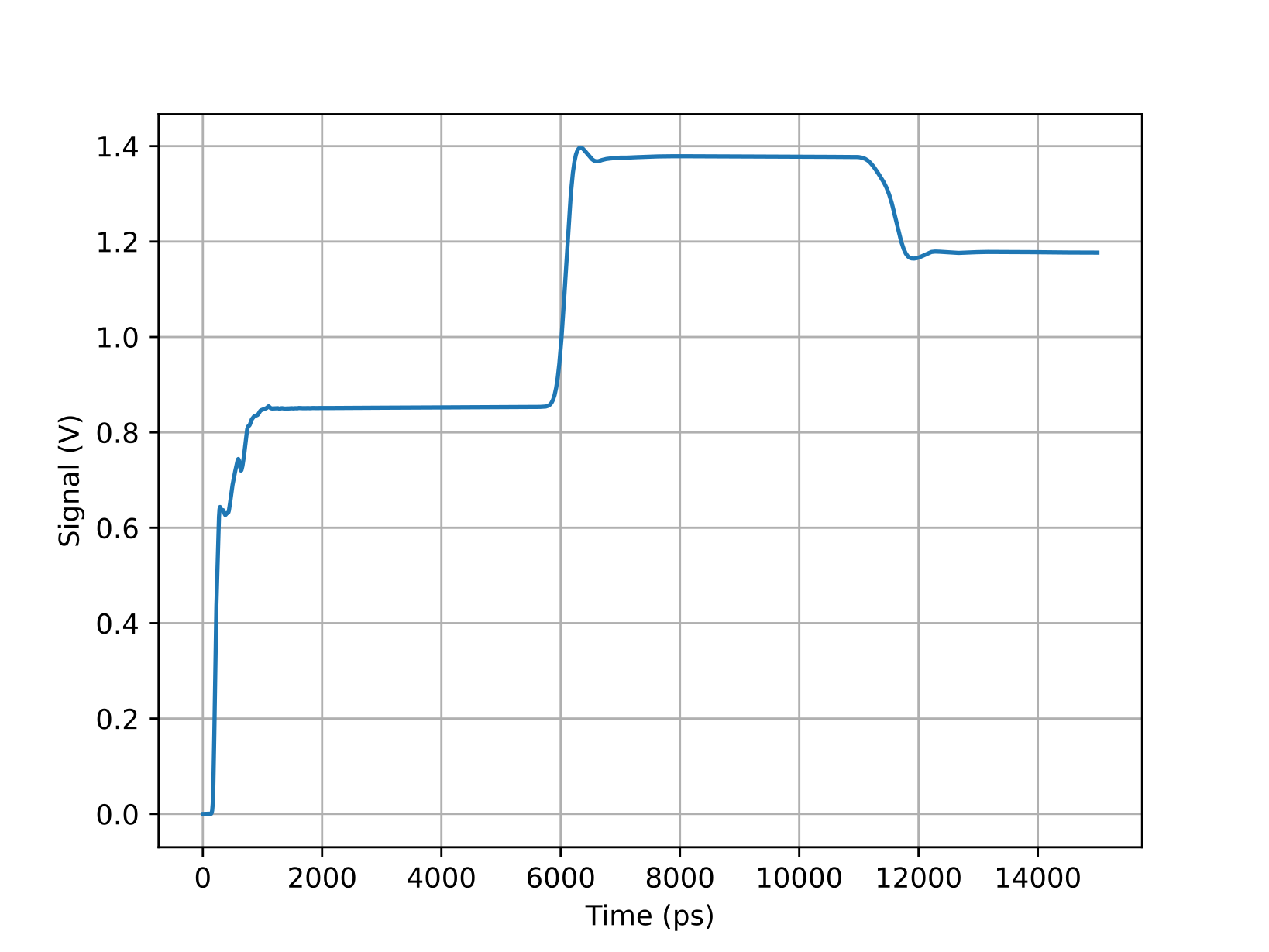
Here’s an example of the resulting waveform, showing a 214 ps rise time.
Here’s what we did.
System Overview
This optimization system includes:
- A parameterized OpenSCAD model for geometry generation.
- A Python simulation that uses Docker to run OpenEMS. Parameters are passed in using a CLI.
- A scoring function that evaluates TDR-like pulse responses.
- An optimizer from SciPy to minimize rise time and other signal artifacts.
- A STL generation step which generates the models from the OpenSCAD source.
- Simulation results stored in timestamped directories for later review.
flowchart LR
    A[OpenSCAD Parameters] --> B[STL]
    B --> C[Docker/OpenEMS Simulation]
    C --> D[Pulse Response]
    D --> E[Score]
    E --> F[Optimizer]
    F -->|Update parameters| A
Simulation and optimization loop structure.
Running a script
docker run -v $(pwd):/home/appuser -t --rm --name openems openems python3 simulation_script.py --maxtime 10e-9
simulation/
├── simulation_script.py
├── caller_cli.py
├── objects/
|   └── ...
├── results/
│   └── {RUN_NAME}_{VARIABLES}_{TIMESTAMP}/
│       ├── et
│       ├── ht
│       ├── port_it_1
│       ├── port_ut_1
│       ├── ...
│       ├── PEC_dump.vtp
│       ├── settings.csv
Calling OpenEMS from a script
The following executes the simulation script and passes in parameters as command line arguments. Use this to step through different parameters, in the next step we’ll use this to setup an optimizer.
def run_simulation(dname, script, kwargs):
    args_ = []
    kwargs.update({
        "dir": str(dname),
        "stl": str(dname / STL_FILE)})
    for key, value in kwargs.items():
        args_.append(f"--{key}")
        args_.append(str(value))

    args = ["docker", "run","-v", f"{base_dir_}:/home/appuser", "-t", "--rm", "--name", "dummy", "openems", "python3", str(script)]
    args.extend(args_)
    with subprocess.Popen(args) as process:
        process.wait()
Adding an optimizer
To optimize we need a scalar score for each run.
Run Score
In our example this is the minimizing the rise time, overshoot, and pulse artifacts of a TDR return. I calculated these using the control library though I’ve also been developing a more tailored alternative here.
import control
import numpy as np

def response_score(x, y, *, bounds=None, weights=None, vdiff_min=0.1):
    if not bounds:
        bounds=(1800, 6000)
    if not weights:
        weights = {"1/RiseTime": 2000, "Overshoot": 500, "Undershoot": 500, "VDiff": 1000}

    mask = (x > min(bounds)) & (x < max(bounds))
    x_bound = x[mask]
    y_bound = y[mask]

    # Ensure we have data after bounding
    if len(x_bound) == 0 or len(y_bound) == 0:
        raise ValueError("No data in the specified bounds.")

    step_info = control.step_info(sysdata=(y_bound, T=x_bound))

    values = {
        "1/RiseTime": 1/step_info["RiseTime"] if step_info["RiseTime"] > 0 else 0,
        "Overshoot": step_info["Overshoot"],
        "Undershoot": step_info["Undershoot"],
        "VDiff": step_info["SettlingMax"]-step_info["SettlingMin"]}

    score = sum([values[key]*weights.get(key, 0) for key in values])
    valid = (np.max(y_bound) - np.min(y_bound)) > vdiff_min
    return int(valid)*score, values, weights
For this project I added a few other options that also optimized on some of the parameters to make the waveguides easier to make. This is easily added so I won’t complicate the example with it.
Choosing an optimization strategy
This usually takes a few steps. For this project I did a rough estimate of the structure using two parallel cylinders. I used those values as the starting values and then ran the simulation for constant steps around those values. This results in 81 simulations (4 parameters with 3 variations: 3⁴ = 81). How long this takes depends on the simulation size but don’t wait around.
import pandas as pd
settings = pd.DataFrame([
    {"name": "dy", "start": 12.7, "min": 12.7, "max": 30},
    {"name": "top_angle", "start": 50, "min": 25, "max": 50},
    {"name": "body_length", "start": 25, "min": 12.7, "max": 25},
    {"name": "base_diameter", "start": 19, "min": 12, "max": 3*INCH/4},
])

# Number of steps for each parameter (can be customized)
num_steps = 3

# Generate value ranges for each parameter
param_names = settings["name"].tolist()
value_grids = [
    np.linspace(row["min"], row["max"], num_steps)
    for _, row in settings.iterrows()
]

parameter_settings = [
    dict(zip(param_names, combo))
    for combo in itertools.product(*value_grids)
]

for parameter_setting in parameter_settings:
    optimize_geometry(args=None, settings=parameter_setting)
After some analysis and eyeballing I chose the values for the optimizer which were tweaked a few more times.
Scipy has a bunch of optimization algorithms, I got the best results using dual_annealing for global optimization.
from scipy.optimize import dual_annealing

x0 = np.array(settings["start"])
bounds = [(line["min"], line["max"]) for _, line in settings.iterrows()]

dual_annealing(optimize_geometry, bounds=bounds,
               args=(settings,),
               maxiter=1000,
               initial_temp=5230.0,
               restart_temp_ratio=2e-2,
               visit=2.62,
               accept=-5.0,
               maxfun=10000000.0,
               x0=x0)
While iterating I got good results using minimize with the Powell method.
from scipy.optimize import minimize
x0 = np.array(settings["start"])
bounds = [(line["min"], line["max"]) for _, line in settings.iterrows()]

res = minimize(
    optimize_geometry, x0, tol=1e-5,
    method="powell",
    args=(settings), bounds=bounds,
    options={"maxiter": 10000})
Let’s now define optimize_geometry, which ties everything together.
Optimization function (optimize_geometry)
This function needs to match the interface expected by scipy and return a scalar value. For reproducibility and debugging, each run stores both the simulation output and its input parameters in a timestamped directory. This lets us go back and analyze all the runs for debugging and for growing some intuition. We also store the weights and the measured values in results.csv.
import time
from pathlib import Path

SCRIPT=Path("simulation_script.py")

sub_dir_ = Path("results").absolute()

def optimize_geometry(args, settings):
    default_settings = {
        "top_angle": 49.5,
        "side_angle": SIDE_ANGLE,
        "dz": 1*INCH,
        "dy": 0.93*INCH,
        "base_diameter": 19,
        "body_length": 25,
    }

    kwargs = default_settings
    kwargs.update({pt: args[i] for i, pt in enumerate(settings["name"])})

    dname = f"simulation_{int(time.time())}"
    dname_local = sub_dir_ / dname
    os.mkdir(dname_local)

    make_model(dname_local, **kwargs)
    df = pd.DataFrame([{"name": key, "value": value} for key, value in kwargs.items()])
    df.to_csv(dname_local / "settings.csv")

    dname_docker = Path("/home/appuser") / sub_dir_.stem / dname
    run_simulation(dname_docker, script=SCRIPT, kwargs=kwargs)

    xv1, yv1 = load_data(dname_local, port="port_ut_1")
    score, values, weights = response_score(xv1, yv1)
    df = pd.DataFrame({"values": values, "weights": weights})
    df.to_csv(dname_local / "results.csv")
    return -1*score
The score is made negative as we are minimizing and our weights are positive.
Make Model
Here I’m using OpenSCAD to generate an STL, which is then used in the simulation. The OpenSCAD model and the simulation connection logic are outside the scope of this post, but here’s the python for a generic set of arguments. You can also do this using JSON if preferred.
The STL geometry is generated with a parameterized OpenSCAD script that models the coupling structure.
def make_model(dname, source_file, stl_file, **kwargs):
    output = dname / stl_file
    arguments = " ".join([f"-D {key}={value}" for key, value in kwargs.items()])
    os.system(f"openscad {str(source_file)} -o {output} {arguments}")
Simulation Script
To keep this post focused, I won’t dive deep into simulation setup details but I’d like to discuss the interface I’m using. I have OpenEMS in a Docker container (You can find the Docker build here: openEMS Docker container) and the tools I’m using are local so this is a little strange. I pass in the arguments through command line arguments using the click library.
@click.option("--dir", "dir_", default=None)
@click.option("-v", type=int, default=0)
@click.option("--zcut", type=float, default=18*inch, help="Make the section above this the surrounding material, chopping off the tines")
@click.option("--zmax", type=float, default=250)
@click.option("--fields", is_flag=True, default=False)
@click.option("--run", type=str, default="simulation_output")
@click.option("--maxtime", type=float, default=10e-9)
@click.option("--e_abs", type=float, default=3.2, help="Dielectic constant of epoxy")
@click.option("--e_dirt", type=float, default=7, help="Dielectic constant of dirt")
@click.option("--k_dirt", type=float, default=0, help="Conductivity of dirt")
@click.option("--stl", type=str, default=os.path.join(os.getcwd(),'./mechanical/pyramid-coupling-with-anvil.stl'))
@click.option("--no_csx", is_flag=True, default=False)
@click.command()
def main(dir_, v, zcut, zmax, fields, run, maxtime, e_abs, e_dirt, k_dirt, stl, no_csx):
    ...

if __name__ == "__main__":
# Change current path to script file folder
    abspath = os.path.abspath(__file__)
    dname = os.path.dirname(abspath)
    os.chdir(dname)
    main()
Summary
This post glossed over the simulation specifics, but it demonstrates how even a small amount of code can drive effective geometry optimization using Docker, OpenEMS, and Python.
This post outlined a lightweight but effective framework for geometry optimization using OpenEMS. By combining:
- Parametric geometry generation with OpenSCAD
- Dockerized simulation runs for clean reproducibility
- Python-based score functions for signal quality metrics
- And global and local optimization via SciPy
A more detailed walkthrough with a sharable version is in the works—stay tuned!